18-Mar-2015: Friction Lab

This lab contained five different experiments involving friction.

Part 1: Static friction

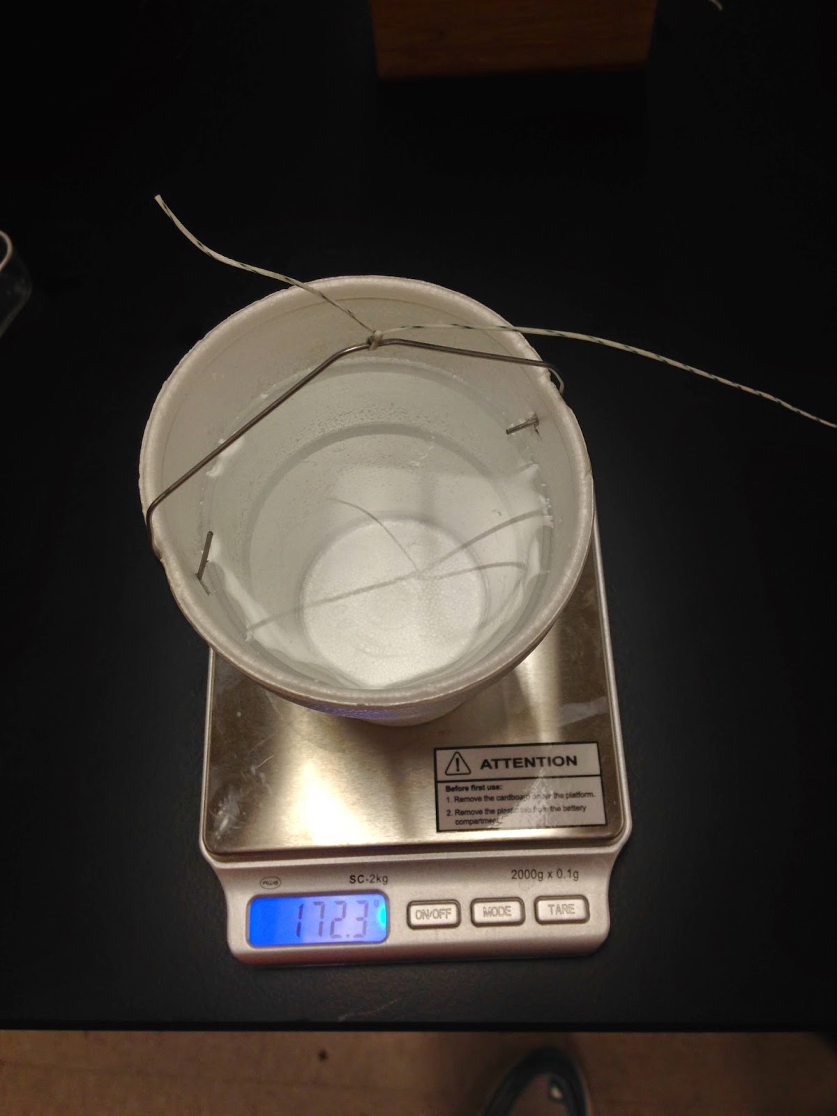
Static friction is the force acting between two bodies when they are not moving relative to one another. In this experiment, we added water to a cup  a little bit at a time until the block just started to slip.

The threshold of motion in this experiment is defined by the coefficient of static friction

u static = f static maximum / N 

since

f static maximum = u static * N

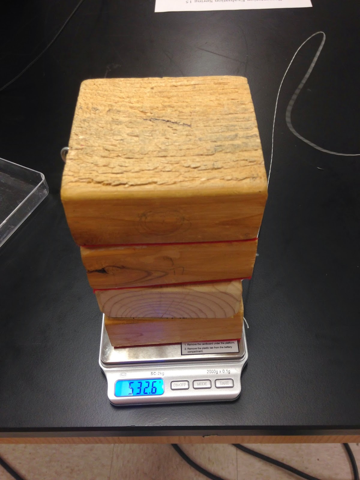
The block has a velvet material. To determine the coefficient of static friction of that material on the table, we need to find its normal force which depends upon its mass.

Mass of One Block

Then we filled the cup attached to the string to find the force that equaled the static friction maximum, or the amount of water it took just before the block moved. We used the mass of the water in the cup times gravity to find the force equal to the static friction maximum.

Mass of Water for One Block

We then repeated this process but after adding a new block onto the block for a total of four trials. 

Mass of Two Blocks

Mass of Water for Two Blocks

Mass of Three Blocks

Mass of Water for Three Blocks

Mass of Four Blocks

Mass of Water for Four Blocks

Using this data we created a data table that first had the mass of the blocks and then mass of the cups of water. We then made a column that represented normal force (mass of block*gravity) and one that represented the static friction force maximum (mass of water*gravity).

(picture of data but my lab partner is laggin it....)

We then graphed the data so that we could find the slope. Therefore, the experiment was successful since the slope showed us the coefficient of static friction for the red velvet on the table surface. 

(picture of graph.....lab partner again...awk)

Part 2: Kinetic Friction

f kinetic = u kinetic*N

Using the logger pro we connected the block to the Force Sensor. We got a second block on top of the first and repeated the experiment until there were three more blocks on top like the previous experiment. The graph below showed the force which equalled the force of kinetic friction since velocity was constant.

(graph)

The data received from the mean of each line was used for the force of kinetic friction which was then divided by normal to get the kinetic coefficient of friction.

(data)

The coefficient of friction was then averaged to be equal to (coefficient).

Part 3: Static Friction From A Sloped Surface

We placed a block on a horizontal surface. After slowly raising one end of the surface, we tilted it until the block started to slip. We then took the angle measurement.

We then used the angle to calculate the coefficient of static friction.

Part 4: Kinetic Friction From Sliding A Block Down And Incline

With a motion detector at the top of an incline steep enough that a block accelerates down the incline, we measured the angle of the incline and the acceleration of the block and determined the coefficient of the kinetic friction between the block and the surface from our measurements. 

Free Body Diagram

Lab with Motion Detector

Coefficient of Kinetic Friction 

Part 5: Predicting The Acceleration of a Two-Mass System 

Using this coefficient of kinetic friction we derived an expression for what the acceleration of the block would be if a mass was hanging from the other end of a pulley. 

Then the actual acceleration was recorded on the graph below.

(picture of graph, if my partner would help...)

Therefore, the percent error was %, a close match. 

12-Mar-2015: Modeling the fall of an object with air resistance

Part 1: Determining the relationship between air resistance force and speed

Air resistance is based on an object's speed, shape and the material it is moving through (type of air).

In this lab we used a simple model to calculate air resistance. We dropped objects from a high enough distance until they reached terminal velocity, where air resistance equalled the speed.

Terminal Velocity 

When acceleration is zero

Using the Design Technology building's indoor balcony, we were able to drop coffee filters from the balcony and use Capture Video to record 1, 2, 3, 4, and 5 coffee filters falling from the balcony.

One Coffee Filter

Five Coffee Filters

As one can see the increased coffee filters are heavier and have an increased terminal velocity. (Not all of the videos made it through email besides these two.)

Part 2: Modeling the fall of an object including air resistance

Using the Capture Video we pin pointed the position of the filter after every frame of the video giving us nice position versus time graphs. We took the slope of each of these graphs when the graph straightened out into a linear graph. The slope was therefore the terminal velocity of each trial. (The data of each graph in the email would not open on my computer.)

We then created a graph with F of resistance versus the terminal velocities found above.

This is the data of force of air resistance and terminal velocity. The F was found using mg, the mass of the filters times gravity. 

mass of coffee filter

(This is where the data for F vs. v would be but my partner is not sending it to me.)

Then we graphed this data to create a curved graph. The graph then had a certain power to it, which we can found using a power fit. The n is shown in the picture below. 

(This is where a graph pic would be but my partner is not responding.)

The equation of the force of resistance is now assumed to have a power and look like this:

F resistance = kv^n (The k term takes into account the shape and area of the shape.)

The model equation may not have "spit out" values close to the terminal values found without experimental data, but this is because our data varied and may have had some human error in taking the position versus time. In the end though, the correlation between velocity and air resistance became clear to how much they are dependent upon each other. The simple model showed us that the air particles that are in the way get accelerated from rest to speed so that the force on the air particles is really the mass of the air in the way. If the weight is added it seems as if the particles will retaliate with equal force, but some particle get out of the way as well creating more varied experimental data.

2-Mar-2015. Sparker Free Fall Lab.

Purpose: To prove that in the absence of all other external forces except gravity, a falling body will accelerate at 9.8 m/s^2.

Experiment: Using the sturdy column (Picture 1), a free-fall body is held at the top by an electromagnet is released and as it falls, its fall is precisely recorded by a spark generator. The marks made at the intervals on the spark-senstive tape attached to the column create a permanent record of the fall.

(Picture 1)

 The series of dots on the paper corresponding to the position of the falling mass are each in 1/60th of a second intervals. We placed a two-meter stick next to the tape, lining up the 0cm mark with one of the dots from the beginning.

Recorded position of the free-fall body (Picture 2)

Add caption

After recording the distance from the 0cm to the next dot, we got a table of data representing the Time vs Distance (Picture 3).

(Picture 3)

The graph of this data is represented below: 

We then made another column that represented the ∆x, the next column was the mid-interval time, and then we used these two new columns to make third column of velocity. 

We then graphed velocity versus mid-interval time to create a scatter graph with a trend line's slope that represented the acceleration. 

The picture shows our resultant calculation of gravity being 9.6218m/s^2 (the slope m in the y=mx+b equation). 

We then recorded the entire classes' gravity results from everyone's experiment to find the standard deviation of the experiment, therefore analyzing the reliability of the experiment. 

The first column values represent the different results from each experiment. The next columns show the manipulations required to result in a 0.2 m/s^s standard deviation in finding gravity.  

The results prove that the experiment is not the most reliable in finding gravity, since the results varied so much.  

4-Mar-2015. Non-constant Acceleration Problem.

Problem: A 5000-kg elephant on frictionless roller skates is going 25 m/s when it gets to the bottom of a hill and arrives on level ground. At that point a rocket mounted on the elephant's back generates a constant 8000 N thrust opposite the elephant's direction of motion. The mass of the rocket changes with time (due to burning the fuel at a rate of 20 kg/s) so that the m(t)= 1500kg -20 kg/s*t.

Find how far the elephant goes before coming to rest.

While using Newton's second law to find acceleration, and then using an equation for the ∆v from 0 to t, v(t) = v + (the integral from 0 to t) a(t)dt, and then deriving the equation once again to find the ∆x give an accurate solution, we found a much easier solution to this problem using excel.

Rather than deriving a complex problem, we used excel to produce the same results by just using the acceleration equation:

a = F/m = -8000 / (650-20t) = -400 / (325-t)

We realized a new way to answer our question, which was by finding the Reimann Sum using excel. The Reimann Sum is an approximation of the area of a region, underneath a curve. The sum is calculated by dividing the region up into shapes, rectangles, to form a region that is similar to the region being measured.

Visualization of Reimann Sum

We then calculated the area for each of these shapes and added them up to get an idea of the larger area, or essentially the integral of a function. We used excel to calculate the many increments needed in finding the most accurate integral.

Beginning of Data Table

The Data Explained:
t: The time gave a time for each acceleration and velocity and position across the data table.
a: This column was formed by using the equation after plugging each time from the time column.
a_avg: This column was found by taking the current row of acceleration plus the previous row and dividing by two to create the length of the rectangle.
∆v: The change in velocity was found by taking the a_avg (length of the rectangle) multiplied by the time increment of 0.05s (width of the rectangle) using the equation ∆v=a-avg*t. The area was therefore considered to be an estimate of the change in velocity (integral of acceleration).
v: The velocity column was found by taking the sum of the original velocity and then each row with the next one from ∆v.
v-avg: This column was found by taking the current row of velocity plus the previous row and dividing by two to create the length of the rectangle once again for another integral approximation.
∆x: The change in velocity was found by taking the v-avg (length of the rectangle) multiplied by the time increment of 0.05s (width of the rectangle) using the equation ∆x=v-avg*t. The area was therefore considered to be an estimate of the change in position (integral of velocity).
x: The position column was found by taking the sum of each row with the next one from ∆x.

We then chose a "small enough" set of ∆t so that when our distance results became more precise. This is when we found that after using the time increment of 0.05 seconds, we got our closest results to the actual solutions of the elephant traveling a distance of 248.7 cm until going into the reverse direction.

The farthest position is boxed in blue on the right. 

In conclusion, we found that same results using excel rather than taking extremely difficult integrals, which was that the elephant travels 248.7cm before reversing direction. 

9-Mar-2015. Propagated Uncertainty in Measurements.

Part1: PreLab: Measuring the Density of Metal Cylinders 

Using Density = Mass / Volume, we will calculate the density of three metal cylinders, one aluminum, one steel, and one copper. The mass scale will have an uncertainty of 0.01 since that is how far it measures. We will also used a Caliper ruler that has a measurement capability of 0.01; therefore 0.01 is the uncertainty factor as well. 

Diameter of Aluminum

Diameter of Steel 

Diameter of Copper

Height of Aluminum

Height of Copper

Height of Steel 

Mass of Aluminum 

Mass of Steel

Mass of Copper

Using these values of diameter, height, and mass, we calculated the density deriving a formula from p=m/V.

Derived density formula

We also calculated the propagated error in each of our density measurements. First we recognized the uncertainty of each measuring tool, adding or subtracting the last tenth of the tool's measuring ability. We then calculated the actual range in error by taking partial derivatives of each variable to find how much each level of uncertainty would actually affect the resulting density.

The partial derivatives of each variable.

These calculations represent the derived densities and their uncertainty deviation.

The calculations for finding density of each cylinder

The real density of each are represented in this table:

(Values acquired from Honors of Physical Science)

We determined that although the measurements are not within the experimental uncertainty of the accepted values, they were pretty accurate. 

Steel's experimental density was 7.75g/cm^3 which had a 0.6% error when compared to the accepted value.

Copper's experimental density was 9.22g/cm^3 which had a 3% error when compared to the accepted value. 

Aluminum's experimental density was 2.74g/cm^3 which had 1% error when compared to the accpeted value. 

Part 2: Determination of an unknown mass

In this experiment, there is a bottle hanging from two strings with different tensions of Force on both sides holding an unknown mass for two masses. Our goal is find the mass of each of the two unknowns. This is a statics problem since the mass is in equilibrium, demonstrated in the picture below. 

Picture of Unknown 1

We then set the vertical forces equal to each other to find the variables necessary in finding the mass. 

The variables included force one, force two, theta one, and theta two

We then found each variable using a spring that measured, in Newtons, the force of tension on the string and another tool to find theta. The spring had an uncertainty of 0.5 N and the protractor had a 2 degree uncertainty or an uncertainty of 0.1pie radians. 

Protractor

Spring

We then found the values to each variable of Unknown 1 and Unknown 7. 

Measured Variables

We then used these values to calculate the mass of each unknown and the uncertainty by taking the partial derivatives of each variable from the equation we used to find the masses. 

Mass and mass uncertainty calculations

In the end, the mass of Unknown 1 was experimentally determined to be 0.746 kg plus or minus 0.0902 and the mass of Unknown 7 was experimentally determined to be 0.723 kg plus or minus 0.0879.