6-April-2015: Work-Kinetic Energy Theorem Activity

Purpose: To measure the work done when one stretches a spring through a measured distance.

First we set up a ramp with a cart, motion detector, force probe and a spring shown below.

The force probe was actually put on after this picture. It was set on the bar and attached to the spring to measure the force of the spring. 

We then opened LoggerPro zeroed the probe and motion detector, a verifying motion was in "reverse direction" so that we could find the slope of a positive graph that represented F against distance. 

To collect data, we stretched out the cart and starting taking data as soon as we let go. After receiving the distance and force data from the probes, we created a graph of Force times distance.

We then graphed Kinetic Energy versus position by finding the mass and plotting (1/2)m"velocity"^2. 

We then put both graphs onto the same graph as shown in the examples below:

As one can see, next we took the integral of the Force times Position graph, which equals the work done by the cart. When compared to the kinetic energy of the KE graph at the end of the increment, one can see in the multiple examples above that the kinetic energy and work are the same but inverse of each other. 

Part 2: 

After looking at a Force vs. Stretch of the rubber band (m) i.e. position graph of a machine, we found the work under the graph to be closely related the kinetic energy calculation. The readings varied with the graph so that our estimated calculations of the area under the integral were off of the real value of kinetic energy. 

30-Mar-2015: Demonstration-Centripetal Acceleration vs. Angular Frequency

Purpose: To determine the relationship between centripetal acceleration and angular speed

An accelerometer was mounted on a disc, with a piece of paper connected to it. The accelerometer was used to measure the acceleration in the x and y direction and the piece of paper was used to pass through a photogate so that the period of rotation of the spinning wheel was recorded.

Measurements Made:

1. Length of time for a period to make a couple rotations

2. The accelerometer reading the rotational speed

3. Distance of the accelerometer from the center of the rotating disk

acceleration = radius * rotational speed^2 (a=rw^2)

radius = 13.8-14 cm

Procedure: 

1. We gave the motor connected to the disk some voltage and recorded the acceleration. We then recorded the period of time using Loggerpro's photogate and the piece of paper sticking out from the edge. 

2. We then received a graph of the acceleration and a data table for the period.

Each Trial: 

1. 4.4 voltage on the motor:

Acceleration: 1.557m/s^2 (mean)

Time: (8 rotations-start time)/8 = (16.461-1.672)/8 = period in seconds

2. 6.4 voltage on the motor: 

Acceleration: 5.074 m/s^2 

Time: (10 rotations-start time)/10 = (10.5305-0.1789)/10 = period in seconds

3. 9.6 voltage on the motor:

Acceleration: 11.89 m/s^2

Time: (10 rotations-start time)/10 = (6.784-0.0534)/10 = period in seconds

4. 10.8 voltage on the motor:

Acceleration: 18.15 m/s^2

Time: (10 rotations-start time)/10 = (5.865-0.377)/10 = period in seconds

Data Analysis:

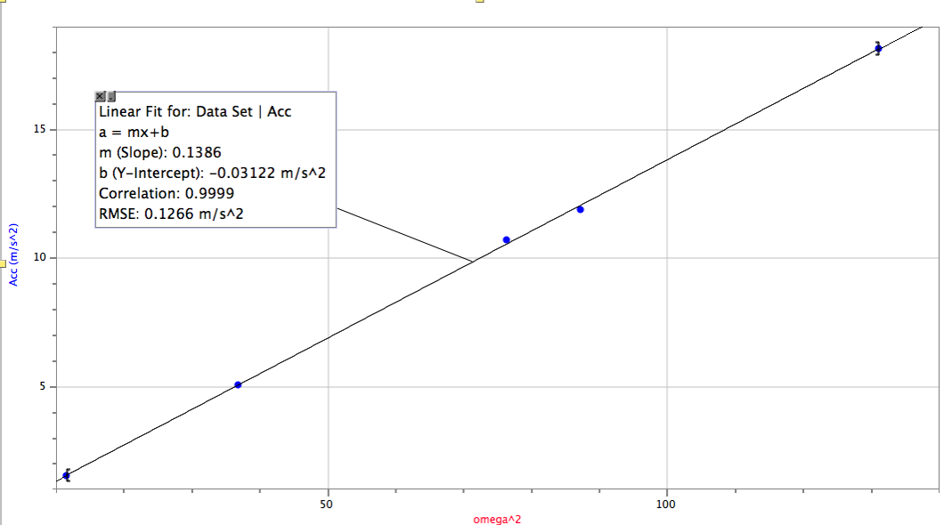
We then plotted and acceleration vs w^2  graph. Acceleration was found using the mean of the data graphs and the omega was found by w=[2(pie)]/T where T was the period that we found. 

After creating a linear fit with our data, we proved that the relationship between acceleration and omega^2 is r since the radius of the disc was 13.8-14 cm and the slope was 0.1386 (meters). 

2-April-2015: Centripetal force with a motor

The apparatus shown below has a motor that spins at an angular speed w. The mass attached at the end of the string is therefore revolved around a centripetal shaft with a radius that increases as the angle alpha increases. The first goal is to find the relationship between w and alpha.

Apparatus at rest

Apparatus in motion

To find w:

1. We first found alpha from looking at the right triangle with hypotenuse L and height 2 which we found by measuring the distance the spinning object was from the ground and subtracting that from the height of the entire apparatus.

2. The height of the spinning object from the ground was estimated by using the tool shown below, where we recorded the height as soon as the spinning object just barely grazed the top of the attached and projected piece of paper. 

Used to find height of spinning object above the ground

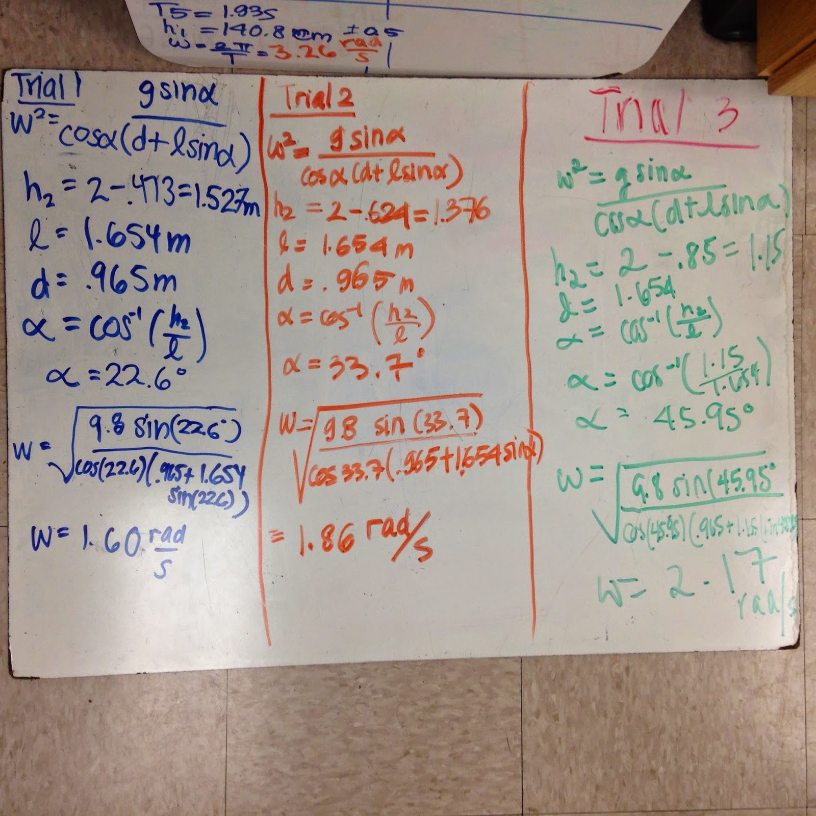
The data from trial one found using these methods are written in red below. The blue is the derived formula for w that uses the variables we just discussed. This is an example of how we used height to find w. 

Calculations to find omega (w)

We then collected multiple values of h at a variety of values of w by increasing the voltage of the motor driving the system's angular speed. To test this model, we then made it our next goal to test the accuracy of these results. We decided to line up our values of omega found by using height with values of omega found by using time. 

Our Data Results:

Each recorded height and time used to find omega

The data shows the time t that it took for one revolution (found by taking the time of ten revolutions and dividing that number by ten). The calculations for finding omega according to the period are clearly shown in each trial. Next we found omega according to the recorded height. 

Calculations used to find omega with height

After using logger pro to also calculate our data, we created a data table with each omega found from each trial. We then plotted the results of both omegas of each trial against eachother in hopes of similar answers or in graphical terms, a slope of 1. 

This was our resulting graph: 

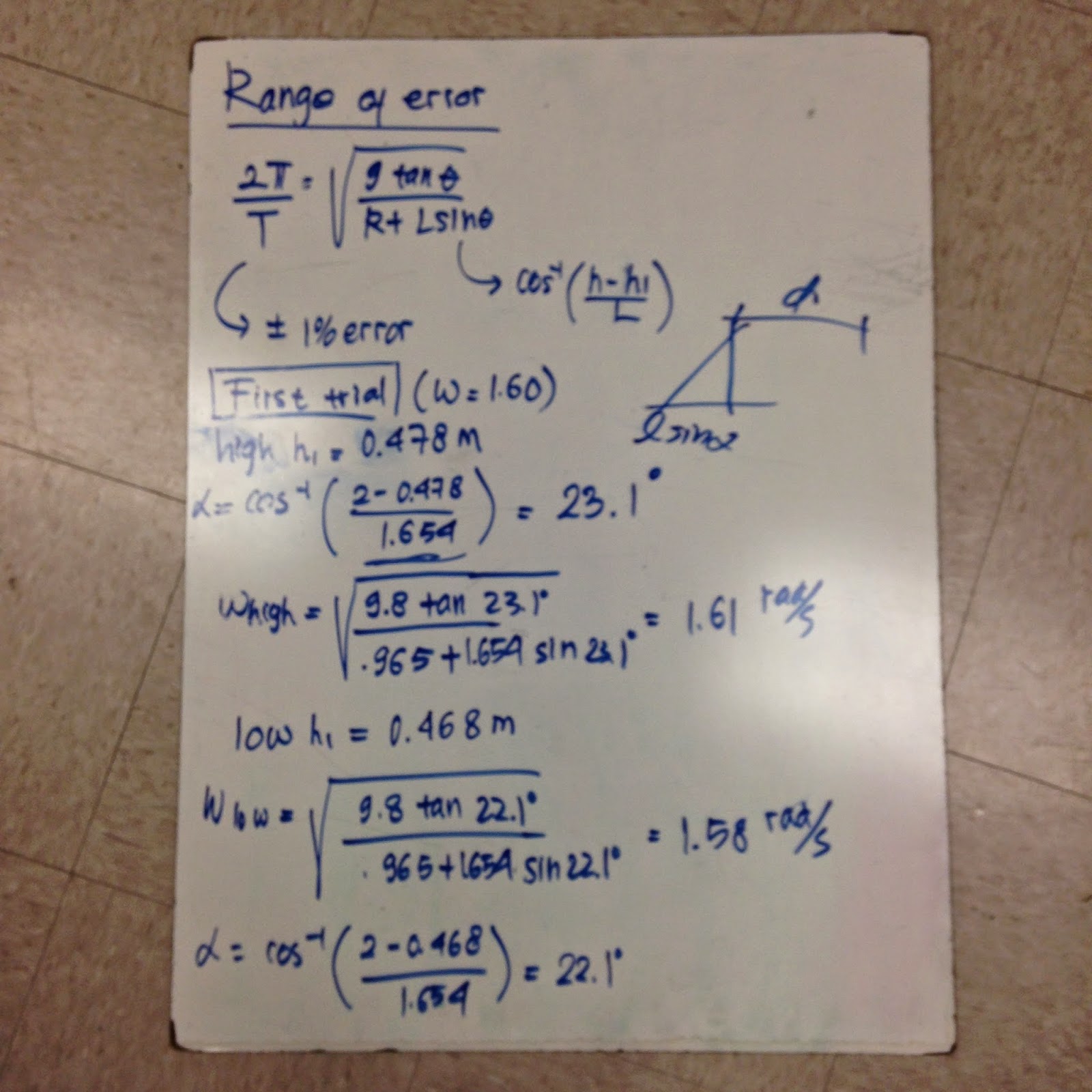
Our results proved successful with a slope of 0.9713. Although these results were close, we had to account for range of error possible in taking the data. After looking at the highest and lowest possible error in recording the time and height, we were able to calculate the highest omegas and lowest omegas from each set of data. 

For example, trial one's range of error:

Range of Error Cacluations

Using these results from the highest to the lowest possible omegas of trial one and trial six we were able to create a range of error by plotting two more graphs. 

Lowest Resutls

Highest Results

In the end, our slope ranged from 0.9824-0.9696, a reflection of a very successful experiment in calculating omega by using the relationship between angular speed and the angle caused by the centripetal force of the rotating apparatus.

23-Mar-2015: Trajectories

Purpose: To use projectile motion to predict the impact of a ball on an inclined board.

Set-up: Aluminum "v-channel" is tilted so that the steel ball goes into another aluminum channel so that there is only a horizontal force when it is launched off the table onto the floor.

Table Set-up

Experiment Part One:

First we found the distance where the ball would land on the ground (not the board yet).

We placed the steel ball from a readily identifiable and repeatable point near the top of the inclined aluminum "v-channel."

Next we taped a piece of carbon paper to the floor around where the ball landed.

We then launched the ball five times from the same place as before and verified that the ball landed in around the same place each time.

We then determined the height of the bottom of the ball from where it launches to the ground, and how far out from the table's edge it lands. (We hung a string with a bobber from the edge to make sure the starting point was accurate.)

Horizontal distance of  0.543 cm

Using this distance and height (s and h), we found the launch speed of the ball from our measurements.

Only the first half (in black) is relevant

Experiment Part Two:

In this experiment, we placed an inclined board at the edge of the table such that the ball would be launched at the same spot as before, but this time it would strike the board, measuring a distance d along the board.

Using the velocity calculated in experiment one and the measured angle (alpha), we then were able to predict the distance d that the steel ball would land on the inclined piece of wood. 

Only the left side is relevant

Using the derived equation we were able to predict distance of 0.5435 meters. 

Our results:

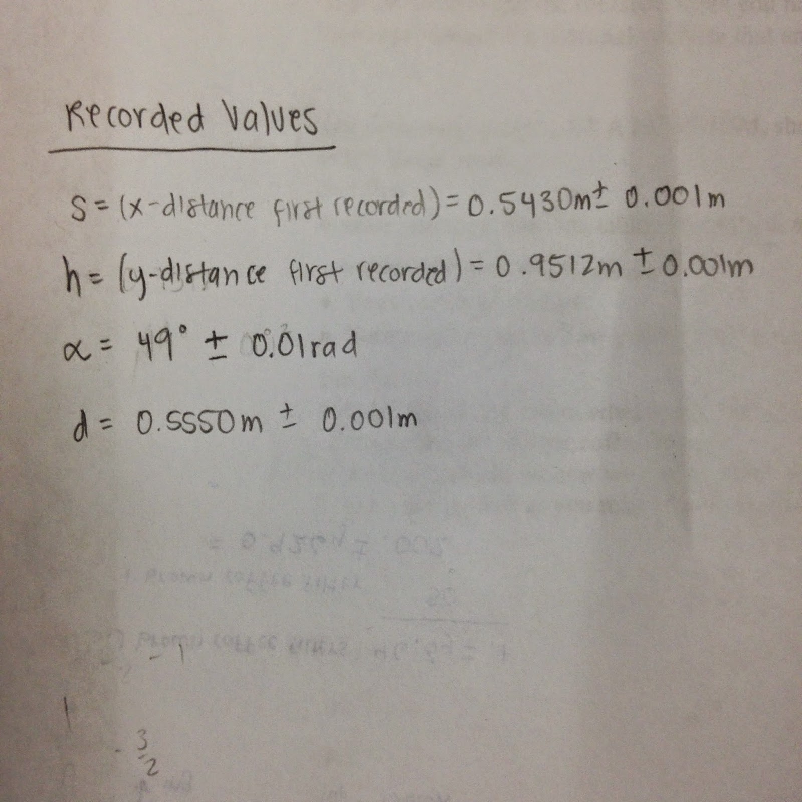
Now that we performed the experiment, the actual distance was 0.5550 meters, which had only a 2% error compared to the prediction. In making our calculations we realized there was a possibility of human error, therefore we calculated the propagated error to give us a range of possible results that the actual results would hopefully lie between. 

Distance Propagated Error of Distance Derived

Overall Propagated Error

According to these calculations, we had a propagated error of 0.009898 meters for d. 

We compared this range to the actual results. 

Predicted and Actual Distances Compared

The actual results were closer to the highest end of the actual results by two thousands of a meter even though they did not actually lie within the range. Overall our calculations allowed for pretty close and accurate results. 

18-Mar-2015: Friction Lab

This lab contained five different experiments involving friction.

Part 1: Static friction

Static friction is the force acting between two bodies when they are not moving relative to one another. In this experiment, we added water to a cup  a little bit at a time until the block just started to slip.

The threshold of motion in this experiment is defined by the coefficient of static friction

u static = f static maximum / N 

since

f static maximum = u static * N

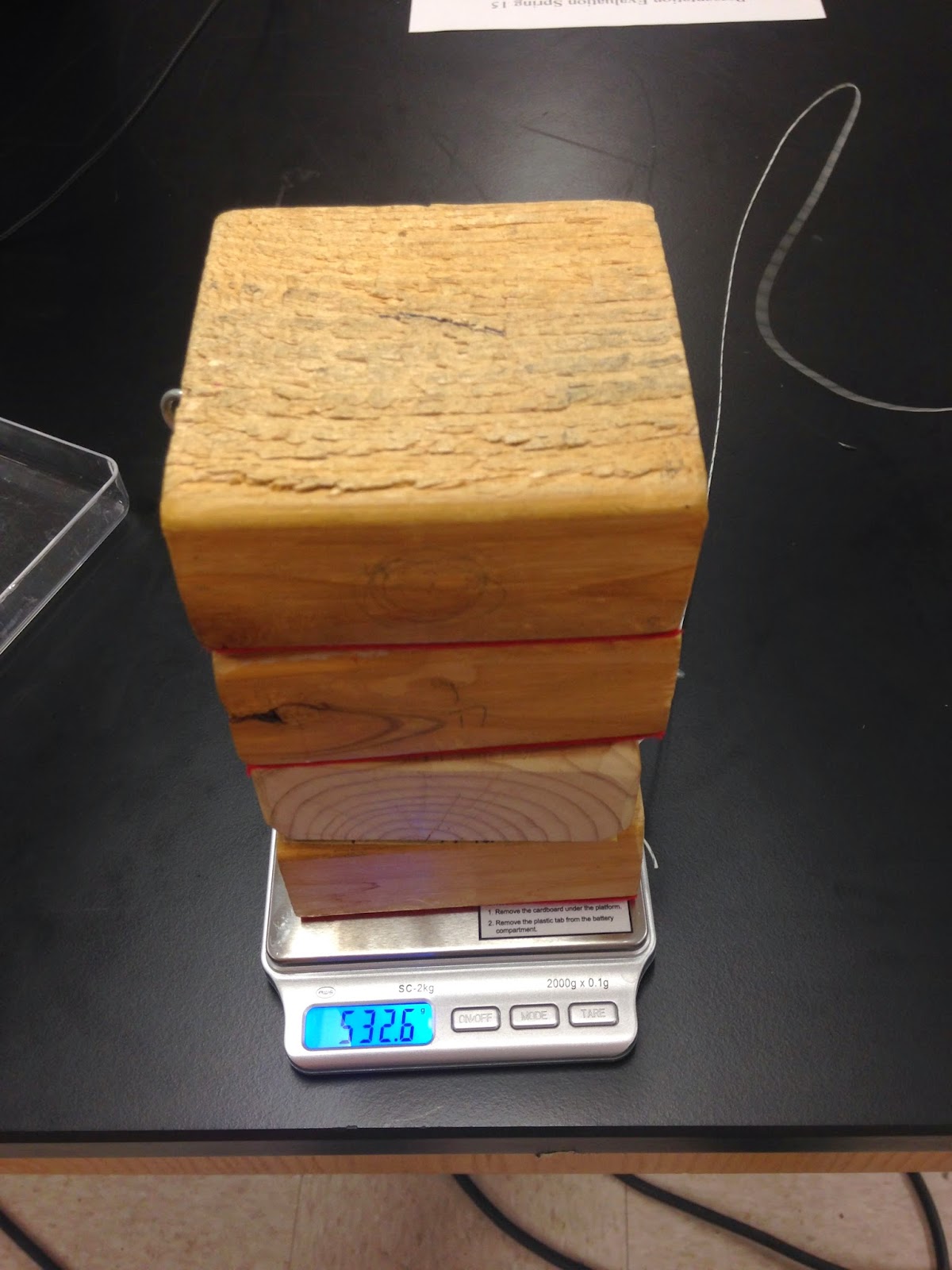
The block has a velvet material. To determine the coefficient of static friction of that material on the table, we need to find its normal force which depends upon its mass.

Mass of One Block

Then we filled the cup attached to the string to find the force that equaled the static friction maximum, or the amount of water it took just before the block moved. We used the mass of the water in the cup times gravity to find the force equal to the static friction maximum.

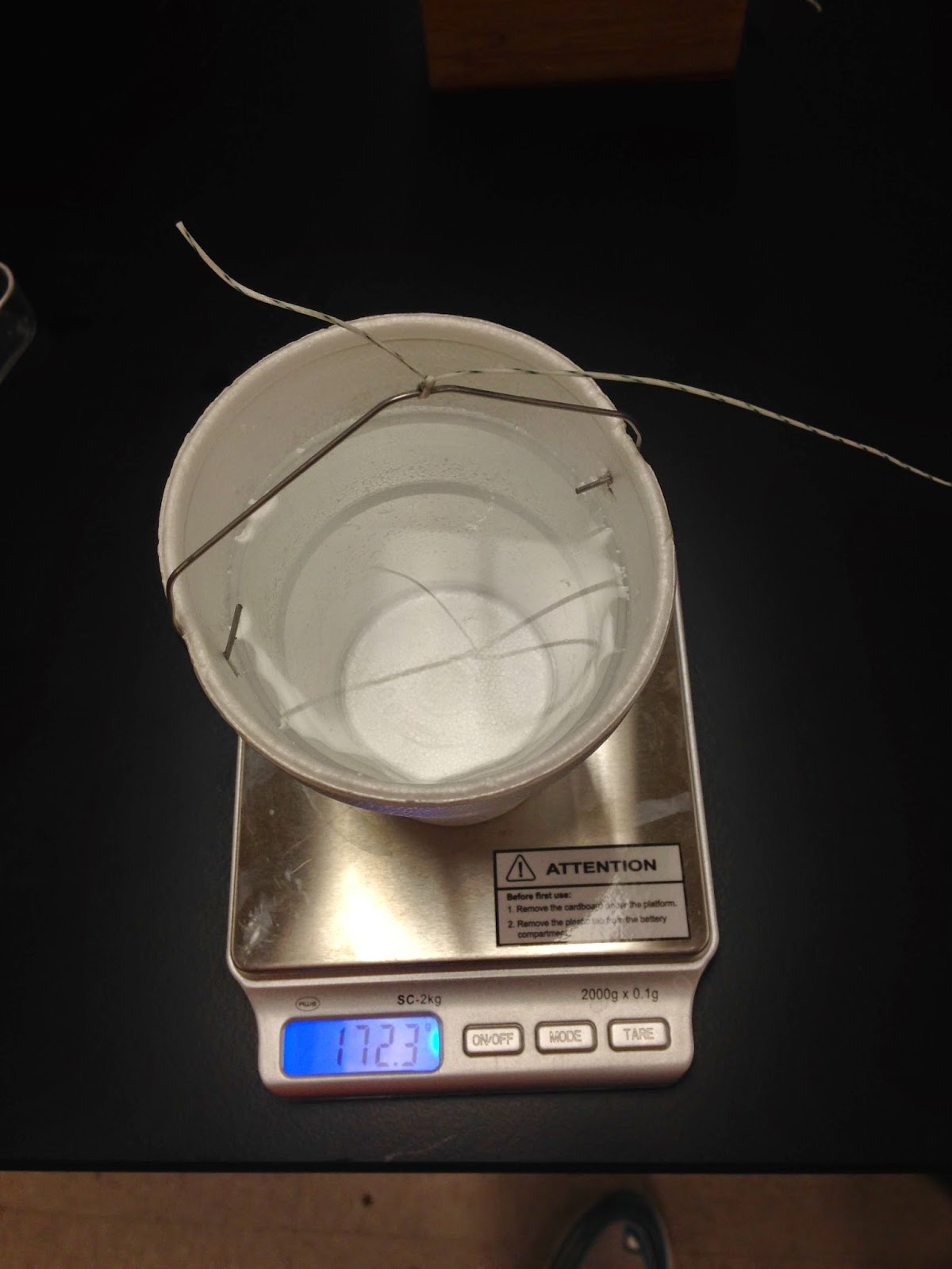
Mass of Water for One Block

We then repeated this process but after adding a new block onto the block for a total of four trials. 

Mass of Two Blocks

Mass of Water for Two Blocks

Mass of Three Blocks

Mass of Water for Three Blocks

Mass of Four Blocks

Mass of Water for Four Blocks

Using this data we created a data table that first had the mass of the blocks and then mass of the cups of water. We then made a column that represented normal force (mass of block*gravity) and one that represented the static friction force maximum (mass of water*gravity).

(picture of data but my lab partner is laggin it....)

We then graphed the data so that we could find the slope. Therefore, the experiment was successful since the slope showed us the coefficient of static friction for the red velvet on the table surface. 

(picture of graph.....lab partner again...awk)

Part 2: Kinetic Friction

f kinetic = u kinetic*N

Using the logger pro we connected the block to the Force Sensor. We got a second block on top of the first and repeated the experiment until there were three more blocks on top like the previous experiment. The graph below showed the force which equalled the force of kinetic friction since velocity was constant.

(graph)

The data received from the mean of each line was used for the force of kinetic friction which was then divided by normal to get the kinetic coefficient of friction.

(data)

The coefficient of friction was then averaged to be equal to (coefficient).

Part 3: Static Friction From A Sloped Surface

We placed a block on a horizontal surface. After slowly raising one end of the surface, we tilted it until the block started to slip. We then took the angle measurement.

We then used the angle to calculate the coefficient of static friction.

Part 4: Kinetic Friction From Sliding A Block Down And Incline

With a motion detector at the top of an incline steep enough that a block accelerates down the incline, we measured the angle of the incline and the acceleration of the block and determined the coefficient of the kinetic friction between the block and the surface from our measurements. 

Free Body Diagram

Lab with Motion Detector

Coefficient of Kinetic Friction 

Part 5: Predicting The Acceleration of a Two-Mass System 

Using this coefficient of kinetic friction we derived an expression for what the acceleration of the block would be if a mass was hanging from the other end of a pulley. 

Then the actual acceleration was recorded on the graph below.

(picture of graph, if my partner would help...)

Therefore, the percent error was %, a close match.